
James Thew - Fotolia
Excel for HR: The essential formulas and functions
Using Excel can benefit HR professionals in various ways, including saving them time so they can work on other tasks. Learn 12 important formulas and functions.

While Microsoft Excel has its limitations, the application can help your HR team analyze employee data using different formulas and functions, save time on rote tasks and increase productivity.
You can use Excel's functions and formulas to sort employees by nationality, calculate hourly rates and sort salaries by department, among other uses. Your HR team's use of Excel can potentially save your company money because so many organizations already use Office 365.
Here's how Excel can benefit HR teams as well as some of the most helpful features and functions.
Benefits of using Excel for HR
Excel offers a number of benefits to HR teams, including the following:
- Empowers data-driven HR. One of the most useful benefits of Microsoft Excel is that it lets HR teams perform a number of ad hoc and basic reporting needs without having to rely on IT. This capability both avoids HR having to wait for requests to be fulfilled and reduces IT's workload, freeing up its time for more complex requests.
- Widely available. Compared to many other applications used in HR, such as a human resource information system, ERP or HR analytics application, Excel is very affordable, regardless of company size. It's often bought as part of Microsoft Office, making it essentially free for most users.
- Accessible to learn. Learning the program is a simple process since a number of Excel learning resources are available on websites, YouTube and social media sites.
- Integrates well. Excel accepts data from any other system or application, making integration easy.
- Offers data analysis and conversion. HR staff can use Excel to quickly generate reports, charts and graphs to help investigate or highlight important information, though this works best for smaller data sets. Excel also handles tasks such as converting HRMS data conversation to something more useful for a presentation. For example, an HRMS may use codes or abbreviations to store data, but a presenter may want to use full words to denote data in a presentation.
Excel features and functions for HR
Some particular Excel functions can help you and the rest of HR accomplish data analysis more quickly. Here are a few to know.
Filtering data in Excel
Filtering data allows you to temporarily hide rows of data that don't meet your criteria, greatly reducing the amount of data displayed in a spreadsheet.
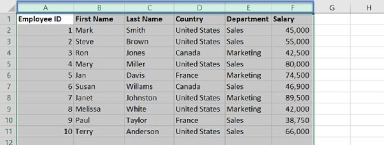
You may want to filter data if many of your company's employees work in different countries and you only want to view American employees' data. You can easily filter out all other countries if the data set includes a country column.
Here's how to use the filter feature.
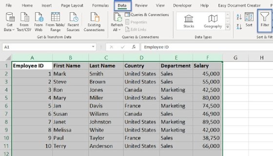
First highlight all the columns with data or select the whole spreadsheet. You can select all the columns in the spreadsheet by clicking inside the area highlighted in green, or you can select only the columns with data, which are highlighted in blue.
Next, enable the Filter feature by selecting the Data menu, then Filter from the Sort and Filter section of the Ribbon.
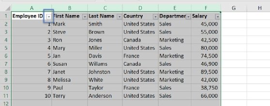
Once you've enabled the Filter feature, a down arrow icon appears next to each entry in the first row of data.
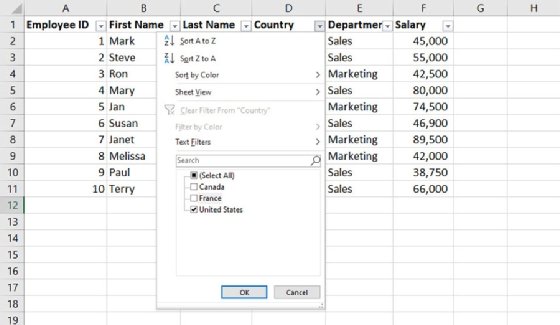
Click on the down arrow in the Country column and deselect all countries except United States. Doing so will hide the rows where the country is anything but United States. Click OK.
You can also use this feature to perform other actions like sorting your data.
Using the data validation feature
The data validation feature is most useful when you want to create a picklist to ensure that any other employees using your spreadsheet only enter valid data in a consistent format.
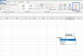
For example, you may have a column in your spreadsheet for the countries in which your organization has offices. You can create a picklist to ensure everyone enters the country name the same way. Otherwise, you may end up with a variety of data entries that have the same meaning but are written differently, such as US, USA and United States. These data variations could make data analysis unnecessarily complex.
To use the Data Validation feature, select Data from the menu, then pick Data Validation from the Data Tools section.
A small window will open. In the window's Allow section, select List. In the Source section, you can either enter a list of values to allow, or you can reference a collection of cells that contains the series of items to display in your list. To reference a range, click the up arrow to the right of the Source field and then select the cell range. Then press Enter to accept the range. The example in Figure 6 displays a hardcoded list of countries.
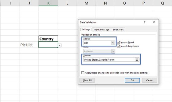
When another user clicks on a cell that contains a picklist, a down arrow will appear next to the field. If they click on the down arrow, they will see a list of valid entries and will only be able to select those entries.
Using PivotTables
You can use PivotTables to quickly analyze data. The tool allows you to drag and drop column names and use predefined functions to perform mathematical computations. HR staff might use PivotTables to compute salaries by country or department or break data down by country and department, among other uses.
To set up a PivotTable, all your columns must have a column header, such as Country, Salary or First Name. If one of the column headers is blank, an error will appear.
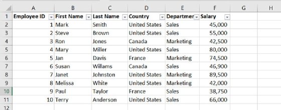
Figure 7 shows an example of salary and country data.
To use the PivotTable feature, follow the steps below.
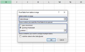
1. Select Insert from the menu, then click on PivotTable in the Tables section of the Ribbon. The window pictured in Figure 8 will then appear.
2. In the Table/Range section, select the data you want to use in your PivotTable. You can select whole columns or highlight the specific section of data you want to analyze. For example, you could select the range A1:F11 for the data pictured in Figure 7.
3. In the Choose where you want the PivotTable to be placed section, indicate where you want to place your PivotTable. The best practice is to put it on its own sheet, since the PivotTable will grow and shrink based on the settings you entered and may overwrite data if you place it near your source data.
4. Next, select how you want to analyze your data. The PivotTable Fields section should display automatically as soon as you click in the PivotTable. If you don't see it, right-click on the PivotTable and select Show Field List. Figure 9 displays the PivotTable Fields window.
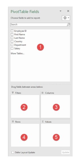
5. Section 1 displays the columns of data you can use based on your selection above. You will drag and drop some or all the column headings into one of the four boxes below, which are items 2 through 5.
6. If you want to filter the data, you can drag a column heading into section 2. For example, if you only want to display data for the United States, you could drag and drop the column heading Country into section 2. The filter section will appear at the top of your PivotTable, and you can select United States.
7. For section 3, you can specify what data you want displayed in each PivotTable column. For example, you may want to place the label Department in this section so each department displays across the top of your PivotTable.
8. For section 4, determine what data you want to display on each row. You may want to place Departments in section 4 instead of section 3 so the departments are placed on each row of the table instead of in separate columns.
9. You use section 5 to perform a mathematical equation with your data. For example, you may want to drag and drop the Salary column heading into this section so you can see the total of every employee's salary. You can also use other mathematical functions in this column. For example, you may choose Count to count the number of employees.
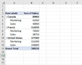
Figure 10 shows an example of how you might format your PivotTable to begin analyzing the data.
Once you have created a basic PivotTable, you can also access additional features that are available from the Ribbon by clicking on the PivotTable Analyze or Design menu items.
PivotTable is a powerful Excel tool because you can easily change the analysis you want it to perform. For example, if you want to reverse the display by having Department follow Country, you simply change the order of the column headings that are depicted in section 4 in Figure 9.
If the company hires new employees, you merely need to refresh the PivotTable and it will display the new data. You refresh a PivotTable by right-clicking on the PivotTable and selecting Refresh.
Excel formulas for HR
Many formulas within Excel can help you analyze data and perform calculations, and the following functions are particularly helpful for HR staff.
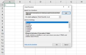
To enter a formula, you can click on the fx icon, which will open the Insert Function window (Figure 11). From there, you can explore the available functions.
Or you can type directly in the cell, starting with the equal sign. You enter the formula as well as any needed arguments, then click enter to get your result.
Here are some useful Excel formulas that HR staff can use to save time and make tasks easier.
SUM. You can use this formula to add the values of several cells. You might use the SUM function to add up employees' salaries.
TODAY(). The Today function returns the current date.
IF. You can use the IF function to perform an action based on the data in one or more cells. For example, you may have a column of data that includes genders, written as M and F, and you want them all spelled out so they read male or female. You can use an IF function to indicate the text that should appear instead.
ROUND. You can use this function to round a number to a specific number of decimal places. For example, if you're calculating hourly rates, you typically want the number to include a maximum of two decimal places.
COUNTIF. You can use this function to count how often a certain value occurs in a range of cells. For example, you may want to count each instance of the word "United States" in the country column to find out how many employees are American.
SUMIF. You can use the SUMIF function when you only want to include a value in a sum if it meets certain criteria. For example, you may only want to add up the salaries of employees who live in Canada.
VLOOKUP. You can use the VLOOKUP function to merge data from one spreadsheet into another spreadsheet. For example, you may have one spreadsheet with employee data, but employee performance data is stored in another HR system. You can use the VLOOKUP function to match employees from your original spreadsheet to the performance appraisals data on another spreadsheet. To do this, you use a unique value that is available on both spreadsheets. For HR data, you should use the Employee ID.
When using the VLOOKUP function, you specify what cell in your original spreadsheet includes that unique data as well as where the function should look for new data; the column that the function should look at when returning data if the IDs match; and whether you want the IDs to have an exact match or a close match. You typically want an exact match when working with employee data.
AVERAGE. This function calculates the average of two or more numbers. You could use the AVERAGE function to figure out an average salary. You can hard code numbers in the function or select a range of criteria cells that you want the function to average.
CONCATENATE. You use this function to merge two data points together. For example, your data may have a column for employees' first names and another for employees' last names. If you want the person's full name to appear in one cell, you can use the CONCATENATE function to merge the values together.
DATEDIF. Although not technically an Excel function, you can use DATEDIF to perform calculations on two dates. For example, you may want to subtract one employee's start date from another's to see how many more years the senior employee has been working at your organization.